SWIM: About Pages

Other research groups have used similar techniques to derive shallow ice maps from MGS TES data (Bandfield & Feldman, 2008), as well as data from Mars Climate Sounder (MCS) on Mars Reconnaissance Orbiter (MRO; Piqueux et al., 2019). These groups used different thermal models, and a different set of heterogeneity assumptions from the SWIM TES analysis. Thus, the final SWIM project analysis combines all three thermally-derived ice maps into a single product that captures some of the uncertainty inherent to these techniques. The combined data product also represents the best map of extant shallow ice derived from thermal data to date.

At a given location on Mars, high and low TI materials respond differently to daily and seasonal changes in sunlight, or insolation. Averaged over the year, high TI surfaces are warmer and low TI surfaces are cooler. The timing and magnitude of temperature changes over the course of a day or a season are also different for different materials. We can predict these differences using numerical models. We determine the TI of the surface of Mars by measuring soil surface temperatures from orbit, and comparing the measured temperatures to model predictions. When we calculate TI from spacecraft temperature measurements, we typically assume that the subsurface is uniform -- i.e. that the surface and the subsurface are made of the same material down to depths of several 10s of meters.

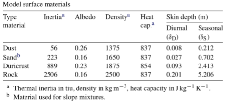
Of course, the real Martian subsurface is complex, especially when ice is present. Figure 1 shows two examples of ice-rich subsurface materials in the Antarctic Dry Valleys. Vertical layering and lateral changes in material types cause the real temperature behavior of the surface to depart from what is predicted by simple, homogeneous models. Figure 2 shows the expected thermal behavior of a uniform, sandy subsurface compared to the thermal behavior of a two-layer surface with dry sand overlying ice-cemented sand. Because we rely on models like the one in Figure 2a to derive thermal inertia, we are really calculating ATI, which can change over the course of the Martian season, depending on how the real structure of the subsurface differs from the simple model (Putzig & Mellon, 2007).

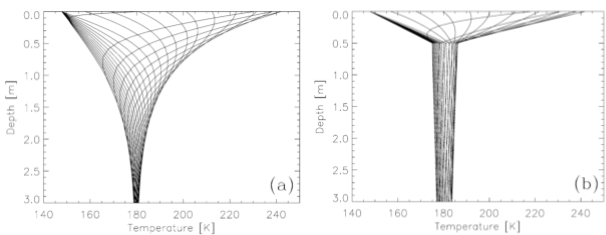
We can use more complicated numerical models of the subsurface (e.g. Figure 2b) to exploit these seasonal changes in ATI and reveal information about the subsurface. In particular, we can look for locations on Mars where seasonal variations in ATI are consistent with a shallow subsurface ice layer.

There are two main data sets we can use to calculate ATI and search for subsurface layering. Data from the Thermal Emission Spectrometer (TES) on Mars Global Surveyor allow us to calculate ATI globally at many times over the course of the year. ATI maps based on TES data have a spatial resolution of ~3 km/pixel. The Thermal Emission Imaging System (THEMIS) on board Mars Odyssey provides us with higher resolution temperature data (100 m/pixel), but less complete spatial and seasonal sampling of surface temperatures. In the SWIM project, we use TES data to make global maps of surface heterogeneity types, including the types of layering that would indicate the presence of ice. We use THEMIS data to do similar analysis on small regions. Areas we target for THEMIS analysis may be locations where other data sets (TES, radar, geomorphology) indicate possible subsurface ice. We can also use THEMIS data to cross check TES results in areas where there is no indication of ice. Using both data sets improves confidence in our results.