
SWIM: About Pages
Curious about what SWIM is all about? Please explore the short articles, written by SWIM Team Members covering various aspects of the datasets included in the search for subsurface water ice on Mars.
Follow us on Twitter!Article List
SWIM Overview
By: Dr. Nathaniel Putzig
Last Updated: 11/02/2020
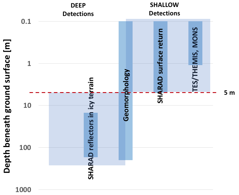
The goal of the Subsurface Water Ice Mapping (SWIM) project is to provide a set of mapping products using existing spacecraft data that delineate subsurface ice in the mid-latitudes of Mars. We aim to identify and map indicators of possible subsurface ice in each data set and use a combination of all data sets to assess the likelihood of ice being present in shallow (< 5 m depth) and deep (> 5 m depth) zones.
Not all existing ice will be identified, since the current data sets impose limits on lateral and vertical resolution as well as sensing depth (Figure 1). In broad terms, the available data sets examine four zones: 1) the surface itself (i.e., to a few microns depth) for imagery and elevation data, 2) within the upper ~1 m for thermal and neutron spectrometers, 3) within the upper ~5 m for radar reflections from the surface, and 4) between ~15 m and several 100 m depths for radar reflections from subsurface interfaces. Geomorphologic indicators of ice span all four zones. Apart from transient ice after a recent impact, there is no ice exposed at the surface in the areas of interest (0 to 60° latitude).
The SWIM Equation
The interpretation of ice presence from these data sets is to a degree subjective and does not lend itself to precise calculation of probabilities. However, some quantification of our confidence in our identification and mapping of ice is warranted and highly desirable for planning future landing sites that rely on the presence of ice for resources or scientific studies. To that end, we have developed the SWIM Equation, produced in the spirit of the famous Drake Equation for conceptualizing the number of civilizations in our galaxy. In the case of the SWIM equation, each of our terms is based on actual measurements and thus we argue that the derived output is a tangible representation of the likelihood of shallow ice.
We begin by defining ice consistency values CX for each data set X that range from -1 to +1, where -1 indicates that a given measurement is inconsistent with the presence of ice. In contrast, a +1 indicates that the measurement is consistent with the presence of ice. A value of 0 means these data are inconclusive or are absent altogether.
| Term | Data Sets | Ice Depth (m) |
|---|---|---|
| CI | All | < 5 and > 5 |
| CN | Consistency of neutron-detected hydrogen with shallow ice | < 1 |
| CT | Consistency of thermal behavior with shallow ice | < 1 |
| CG | Consistency of geomorphology with shallow and deep ice | All |
| CRS | Consistency of radar surface echoes with shallow ice | < 5 |
| CRD | Consistency of radar dielectric properties with deep ice | > 5 |
In assessing the composite ice consistency CI of all data sets, we started with a “hands-off” approach wherein we chose not to apply any weightings or separation by sensing depths during the first season of SWIM (2018-2019):
In assessing the composite ice consistency CI of all data sets, we started with a “hands-off” approach wherein we chose not to apply any weightings or separation by sensing depths during the first season of SWIM (2018-2019):
CI = ( CN + CT + CG + CRS + CRD ) / 5
Our northern hemisphere products available since 2019 use this introductory formulation of the SWIM Equation. In our second season of SWIM (2019-2020), we have introduced a new approach wherein we provide separate equations for three depth zones: 0-1 m, which is dominated by neutron and thermal spectrometer data; 1-5 m, which is dominated by shallow geomorphic and radar surface-return data; and >5 m, which is dominated by deeper geomorphic and radar subsurface dielectric data. To enable this approach, we divided the mapped geomorphic landforms into two groups corresponding to ice presence above and below 5 m depths, producing terms CGS and CGD. In addition, we introduce weighting factors sY, the shallowness of method Y, which is determined by dividing the depth of interest for each equation by the sensing depth of each method. Thus, for the first depth zone, we have:
CI[0-1m] = ( sNCN + sTCT + sGSCGS + sRSCRS ) / (sN + sT + sGS + sRS )
= ( CN + CT + 0.2*CGS + 0.2*CRS ) / 2.4
where:
sN = 1 m / 1 m = 1
sT = 1 m / 1 m = 1
sGS = 1 m / 5 m = 0.2
sRS = 1 m / 5 m = 0.2
For the second depth zone, we have:
CI[1-5m] = ( sGSCGS + sRSCRS + sRDCRD ) / ( sGS + sRS + sRD)
= ( CGS + CRS + 0.3*CRD ) / 2.3
where:
sGS = 5 m / 5 m = 1
sRS = 5 m / 5 m = 1
sRD = 5 m / 15 m = 0.3
For the third depth zone, we have:
CI[>5m] = ( sGDCGD + sRDCRD ) / ( sGD + sRD )
= ( CGD + CRD ) / 2.0
where:
sGD = 15 m / 15 m = 1
sRD = 15 m / 15 m = 1
This formulation of the SWIM equation is by no means the only approach possible, and other methods may be brought to bear, depending on one’s goals.
Example 1: From a thermal perspective (represented by the term CT above), the detection of buried high thermal inertia material is consistent with the presence of ice, and so would be awarded a positive value. On the other hand, detections of buried low thermal inertia material is inconsistent with the presence of ice and would be awarded a negative value accordingly.
Measurement Caveat: A buried high thermal inertia detection is also consistent with the presence of rock. Hence the need for multiple data sets.
Example 2: In the case of radar surface returns (CRS), low power measurements indicate low density material which is consistent with the presence of ice (and so would be awarded a positive value), whereas a high power return is inconsistent with the presence of ice (would be awarded a negative value) and likely indicates high density material such as rock.
Measurement Caveat: A low power return is also consistent with the presence of non-ice low density material such as thick (> 1 m) accumulations of dust.
Taking the two examples above, we see that a positive value for either CT or CRS in isolation is not a unique detection of ice by itself. The power behind the SWIM Equation is that it integrates multiple measurements to build confidence in the detection of ice. Within this in mind, we see that for a given locale, a buried high thermal inertia measurement in addition to a low radar power return are inconsistent with the occurrence of either buried rock or thick dust layers, and instead they argue strongly for the presence of ice.